Neural ODEs

2025-01-28

I implemented neural ordinary differential equations for one of my ESA ML Community talks from scratch, together with my colleague at the time Lorenz Ehrlich. Neural ODEs represent the hidden states of a neural network in a more "continuous" manner. Instead of the neural network generating the hidden states and output directly, the idea is to use the neural network to generate the hidden state's derivatives, serving the role of a model of the hidden state dynamics. Then an arbitrary ODE solver can be used to compute the hidden states by solving the resulting differential equation.

The implementation is pretty straight forward, we just need to build a neural network with any architecture, and have any ODE solver compute the solution for the hidden states dynamics equation. In this case I implemented the regular and adaptive versions of the Runge–Kutta–Fehlberg solver, known as RKF45 or RK45. Since we are working in the context of machine learning, we want to be able to fully utilize the potential of the GPUs, solving batches of ODEs at a time. The interesting challenge here was the implementation of the adaptive solver, because due to the adaptive step, solutions to different ODEs may be computed at different times, because the solution is computed in a constrained time frame, requiring different number of steps. I solved it by masking ODEs that haven't reached the final time step, and returning the batch of solutions when the mask tensor is fully filled with ones.

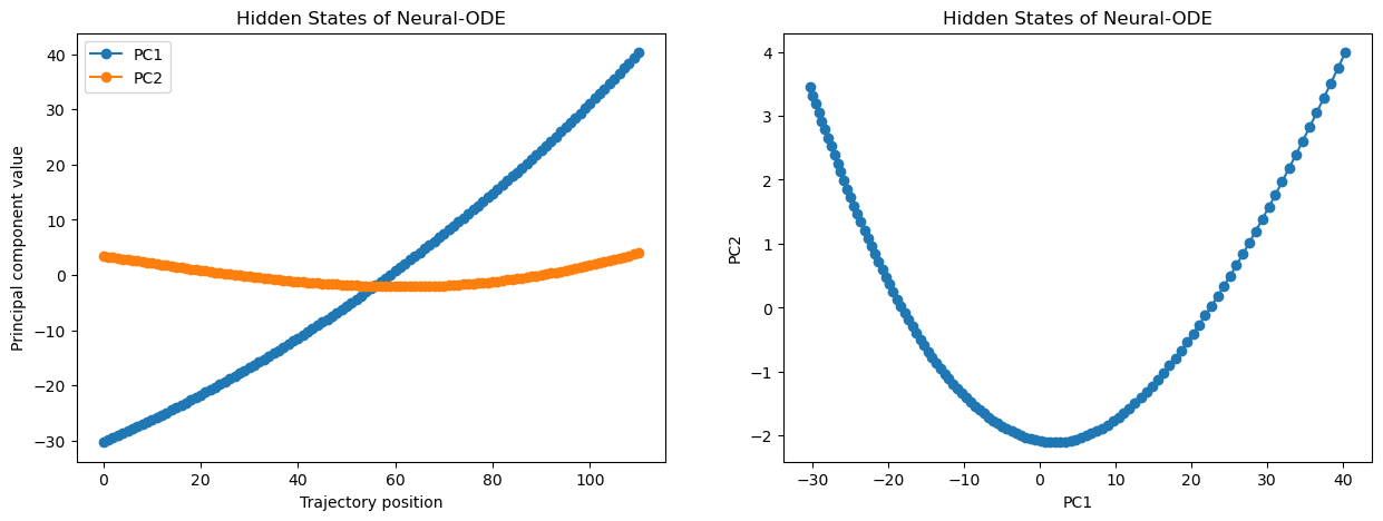
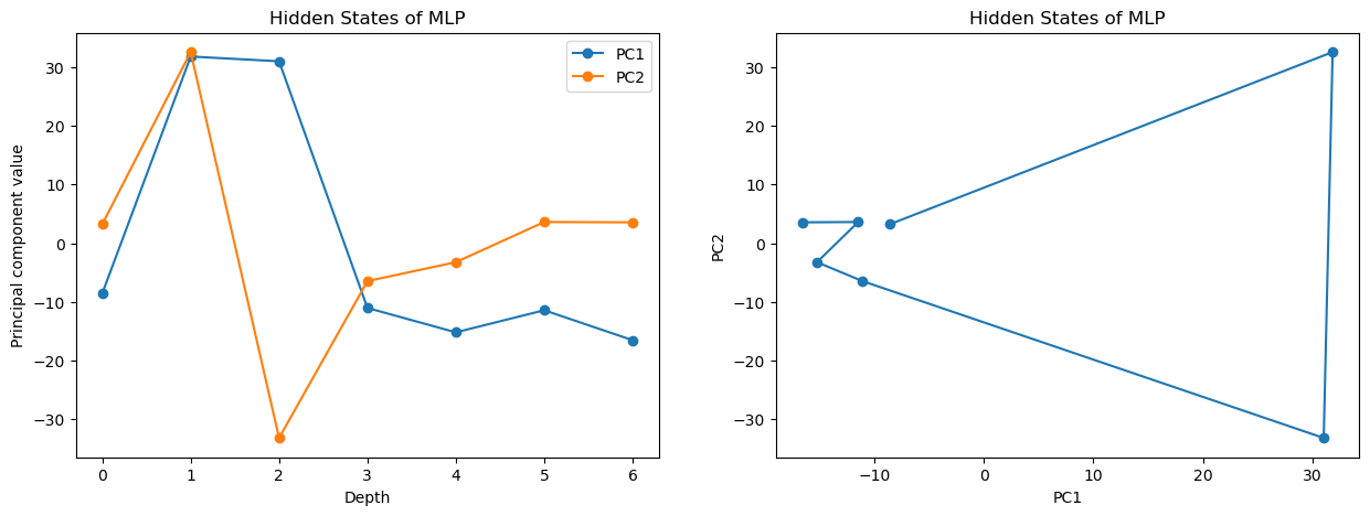
To visualize the core feature of neural ODEs - the continuity of their hidden state, I trained a typical MLP and a neural ODE, with a smaller MLP describing its dynamics on the MNIST dataset. Then I computed the first two principal components on their hidden states while computing inference for a random input. Here you can see the hidden states of the MLP:

And here for the neural ODE, you can see how much smoother and "continuous looking" the hidden state appears to be.